Masters of Engineering Project: GraphLily - Accelerating Graph Linear Algebra on HBM-Equipped FPGAs

The purpose of GraphLily is to accelerate sparse matrix linear algebra computations on a Xilinx Field Programmable Gate Array (FPGA) by leveraging the benefits of High Bandwidth Memory (HBM). Most matrix multiplications can have long execution times due to their O(N²) complexity. To address this, we convert between sparse matrices, matrices filled with many zeroes, and dense matrices, matrices where all zeroes have been removed.

While kernels for sparse and dense matrix multiplication have already been implemented, my project aims to adapt these existing kernels with HBM and extend the design to incorporate a multi-tenancy system. This system allows two users to input their own matrices and perform computation on a new combined matrix to test if there is a performance speedup or deficit because of this combination.

The hardware accelerators can benefit from HBM due to the significantly higher data transfer rate over the standard Double Data Rate (DDR) memory onboard the FGPA, as well as their ability for parallel memory accessing, meaning multiple memory transactions can occur simultaneously. In the initial phase, we will incorporate 16 of the 32 HBM memory channels into our design. Once successful, we intend to include up to 26 of the 32 HBM memory channels as 6 of the channels are required for other processes that benefit overall system performance.

Ideally, with the added HBM channels, once we incorporate this design, we hope to increase our performance from 230 MHz to 275-285 MHz, which is almost as fast as the FPGA will allow: 300 MHz. This is important as data sets continue to increase in size, and without creating new ways to compute this data, users will be forced to wait for much longer times. With the multi-tenancy system and HBM implementation, we hope to optimize performance as much as possible, given the hardware specifications, and further enhance the scalability and efficiency of sparse matrix computations on FPGAs.

Graphing is a universal representation of data that shows relationships and connections. Subsequently, graph processing can be utilized for a diverse range of fields. One of the main issues with graph processing, however, is that most processes are typically bound by memory, due to a low compute to memory access ratio. This has a direct result of bottlenecking graph processing and slowing down the overall execution time. High-bandwidth memory (HBM) has the potential to fix this low compute to memory access ratio. Compared to Double Data Rate (DDR) memory, HBM delivers significantly higher bandwidth over DDR memory, ideally allowing for multiple memory channels to service memory concurrently. We have seen HBM memory make its way to consumer goods like AMD Graphics Processing Units (GPUs) and Field Programmable Gate Arrays (FPGAs) from Intel and AMD. This project makes use of the AMD Xilinx FPGA. Since the Xilinx FGPA has HBM already on board, we can utilize this hardware to speed up the overall process, accelerating graph processing.

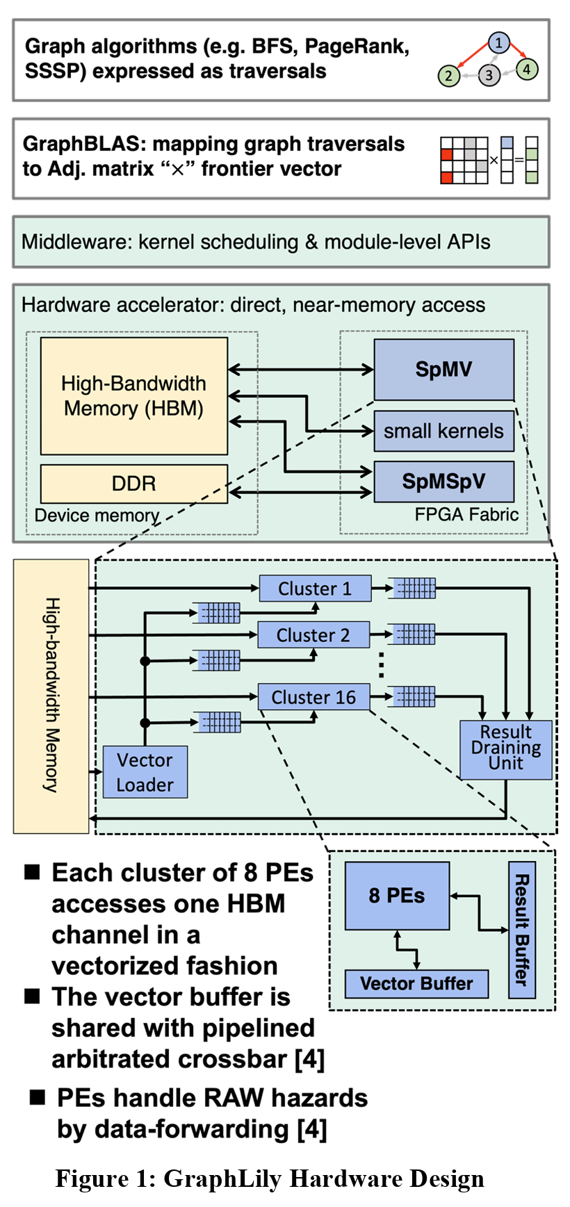
GraphLily¹, which is the graph linear algebra overlay the PhD students have already created aims to provide efficient acceleration of graph processing. To do this, two kernels have been implemented: Sparse-matrix dense-vector multiplication (SpMV) and Sparse-matrix sparse vector multiplication (SpMSpV). The intended use case of these two kernels is to use both together, efficiently switching between kernels depending on the operations needed for a specific algorithm. To accomplish this with HBM, the SpMV accelerator stores the sparse matrix in a customized format that allows for vectorized accesses in the HBM channels. The SpMV accelerator also allows for a scalable on-chip buffer design that replicates vectors and banking to feed many processing elements. On the other hand, the SpMSpV accelerator is designed to read matrix information from regular DDR memory as to not compete with the SpMV accelerator, cutting down on the HBM bandwidth as SpMSpV is faster than SpMV when the input vector has high sparsity, meaning many vector indices are zero.¹

GraphLily is based on GraphBLAS, an open-source library that defines the standard building blocks for graph algorithms of sparse linear algebra. GraphBLAS enables graph algorithms to generalize SpMV and SpMSpV to have customizable binary operators, allowing for the algorithms to use the shortest path algorithms when calculating the distance between vertices in the vector.

HBM is purposely targeted for these applications due to linear algebra computations requiring a lot of bandwidth in terms of memory. As the matrices grow, the overall size in memory grows proportionally. As a result, being able to feed the accelerators as fast as possible is of utmost importance. HBM also allows for a high degree of parallelism, meaning multiple memory accesses can occur simultaneously. This parallelism can greatly increase performance as it requires less time to gather all the necessary information for the specified computation.

In previous versions of GraphLily, the team was successfully able to implement 16 channels of HBM for their design, though when upgrading to a new generation of hardware, these channels no longer work in their design. A reason for this happening is the change in how the FGPA chip handles kernel configuration and physical plotting of the kernels on the chip. The new hardware initially had an issue where the kernels would not fit on the chip, as the place and route tool onboard the FPGA required more hardware resources to fit the design. This means that the required hardware for implementing the SpMV and SpMSpV kernels would need more space on the FPGA than what the chip had available. While this has been fixed, this fix changed how the HBM is configured and utilized in the hardware. Initially, my task was to help fix the hardware challenges with the HBM and help the team understand some of the issues surrounding the configuration of the memory channels.

Once we were able to incorporate all the HBM channels into the design, my focus shifted to creating a baseline design for a multi-tenancy implementation, where two matrices could be combined and produce a single, larger matrix. The reasoning behind this is twofold: understand the performance gains or deficits created by combining two matrices together and if there are beneficial performance gains, implement this combining matrix functionality into a future implementation that operates on scheduling with OpenCL.

To accomplish my goal of connecting the HBM channels in our design, there are 3 steps we plan on taking. I mainly focused on ensuring correct functionality at the software emulation level. By testing with software emulation, I can be sure that the functionality of the test cases for both the SpMV and SpMSpMV would still work when pushing the design through hardware emulation and the actual hardware design. However, due to issues with the SpMSpMV kernel, we are currently unable to properly use this design, even in software emulation, so this year, I’ve been focusing only on the SpMV kernel and ensuring correct functionality. Before touching the decisions made for implementing the design changes, I want to focus on the hardware design and how it works to provide more context.

The diagram below outlines the basic structure for the hardware accelerator. As explained previously, the SpMV kernel only communicates with the HBM memory. Since we are computing spare matrices with dense vectors only, we can take advantage of the extra bandwidth to execute computations faster. As the diagram also explains, since the hardware is designed to be near the memory and have direct memory access, there is lower latency that traditional hardware, like a consumer computer system, where memory operations are handled by the main processor, usually the core processing unit (CPU). In these systems, when an application requires access to memory, the CPU handles the load and store commands and then sends the memory values to the application in question. However, with our design, the hardware accelerator can independently poll the memory, eliminating the “middleman”: the CPU.

Additionally, with the SpMV kernel, we separate this logic into 16 clusters, each containing 8 individual processing elements (PEs). The reasoning for 16 clusters is directly correlated to the number of HBM channels being used in the design. If 32 HBM channels were connected, the design would then contain 32 clusters, each with 8 PEs. Once computation is completed for each of the individual PEs in a single cluster, the results generated are passed into the Result Buffer. This buffer is designed to hold onto the result until all the other PEs have finished their execution of the current task, and once everything has completed, all the results are passed into the Result Draining Unit. The Result Draining Unit handles the reconstruction of the result when being passed back to the HBM, to ensure correct structure and results as to not output incorrectly formatted data, i.e., where the results are correct but in the correct order.

When performing software emulation, the results are simulated depending on the number of HBM channels in mind, which allows for testing correct functionality. To further explain how we test this, the image below in Figure 2 shows a simple diagram of how the matrices are setup, as well as how they are separated to their respective PEs.

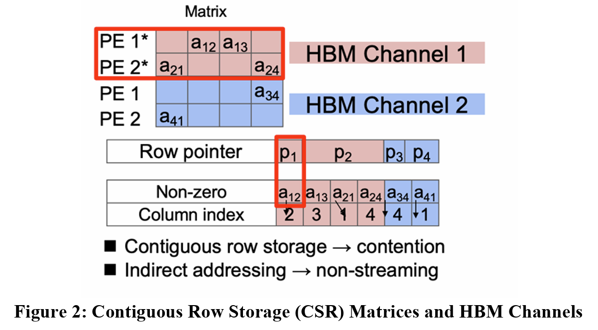
CSR matrices are a type of matrix processing that helps minimize the required space of matrix, allows for computation larger input matrices that wouldn’t be possible otherwise. However, the image above highlights one potential issue that needs to be addressed to make these CSR matrices more friendly for HBM. The current representation shows a load imbalance between HBM Channel 1 and Channel 2 as it causes contention between PE 1 and PE 2. Both PEs require access to the first HBM channel, and while HBM allows for multiple memory accesses at the same time, that’s not possible on a single channel. In this case, PE 1 and PE 2 will need to wait on each other, creating a dependency. To compensate for this, we can modify which HBM channels access which parts of the matrix. Figure 3 below highlight this change.

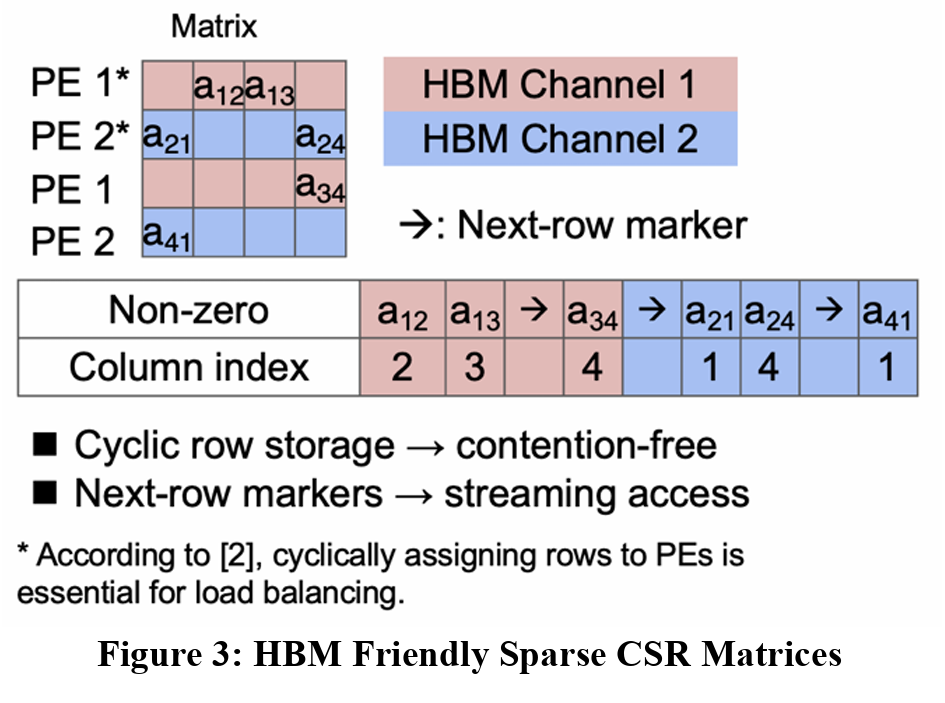
This change helps eliminate the load imbalance previously seen. Now, the first instances of PE 1 and PE 2 both contain 2 elements each, and the second instances of both PEs compute on one element. However, now that these PEs have their own HBM channels, they no longer are dependent on each other, allowing for faster communication with the memory and faster overall execution.

When implementing more HBM channels in the design, I needed to be mindful of which kernels would receive how many additional channels. With different implementations and rounds of testing, I was successfully able to implement up to 26 HBM channels passing with software emulation. This version contained 2 additional channels in sub-kernel 0 and 4 additional channels in sub-kernels 1 and 2. In total, sub-kernel 0 contained 6 HBM channels and sub kernels 1 and 2 contained 10 HBM channels each. I verified these results by successfully passing all SpMV test cases in software emulation, and the next steps, for future designs, would be to implement this during hardware emulation as well as passing on the hardware after place and route.

To aid in ensuring correct functionality for the SpMV kernels when more HBM channels are included, I created two Connected Components test benches. These test cases passed software evaluation, so future implementations could use these test cases in the future.

Once additional HBM channels were successfully implemented, the focus switched to creating a multi-tenancy design, where users can submit more than one matrix at a time to improve overall throughput. We hope that we can save time for the users as there is latency incurred with each computation. The latency is caused from the sending and receiving of the data from the host device. Since this FPGA is connected to a server through a PCIE connection, any input data is sent to the main system, which is then sent to the FPGA. As a result, the main system, the host, sends the data from the host to the device. Once the matrix vector multiplication has completed, the result then must be sent from the host back to the device so the user can access their results. This is where the multi-tenancy idea comes in. If a user submits two matrices that normally would be operated on sequentially. This means the first matrix gets sent and loaded on the FPGA, the FPGA generates the output, and the result is sent back to the host, all before the second matrix can be executed. However, if we could combine the matrices together and operate on them in a single run, maybe there would be a performance benefit. With this idea in mind, the baseline design consists of creating a large matrix from two input matrices. As shown in figure 4 below, we accomplish these by creating a diagonal matrix.

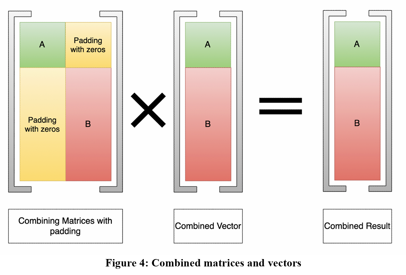
As illustrated above, the diagonal matrix requires padding with zeros to ensure correct functionality and results. By padding with zeros, we can ensure that data is not corrupted by incorrect values and since we are dealing with CSR matrices, we don’t need to compute over those indices where the values are zero.

It’s important for the design to also combine the test vectors for each user’s design. My current implementation calls a custom matrix vector multiplication that splits the computation based on the input matrices. Specifically, when computing over input matrix A, I ensure that the multiplication between the matrix and the vector only executes over the number of columns in matrix A. In other words, if matrix A is a 10 by 10 matrix, with 10 rows and 10 columns, the combined matrix and test vector will loop through the computation and stop each loop iteration at the 10th row in the test vector. When computing the result for matrix B, I then require the execution to start at the beginning of the second matrix’s first row. This ensures that the result for the matrix vector multiplication of input B is not skewed by the data from input A. This is critical as if not done, the results of the combined vector result will be incorrect not only for output A but output B as well.

For the evaluation section, it is important to note that these tests were run on a design incorporating only 16 HBM channels. With 16 channels, both SpMV and SpMSpV perform the correct functionality, though when more HBM channels are created, the SpMSpV kernel produces the incorrect output values. Another PhD student is currently working on fixing this functionality, so I did not aid in helping debug the current implementation’s bugs.

To test the benefits of this multi-tenancy implementation, I combined two input matrices together: dense_32 and uniform_10K_10. I chose these two matrices as the dense_32 matrix is a CSR matrix of size 32 by 32, while the uniform_10K_10 matrix is a CSR matrix of size 10,000 by 10,000. Ideally, it’s important to know if these differing sizes will affect the overall execution time in terms of cycles. For my tests, I combined two dense_32 matrices, two uniform_10K_10 matrices, dense_32 and uniform_10K, and uniform_10K_10 and dense_32. The following table and figure below outline the overall execution time in terms of the number of cycles needed for the execution.

Input Matrices	Cycles
Dense_32	294
Dense_32	308
Combined Dense_32 and Dense_32	308
Uniform_10K_10	3276
Uniform_10K_10	3360
Combined uniform_10K_10 and uniform_10K_10	6317
Dense_32	308
Uniform_10K_10	3150
Combined dense_32 and uniform_10K_10	3185
Uniform_10K_10	3241
Dense_32	294
Combined uniform_10K_10 and dense_32	3304

Table 1: Number of Cycles for each matrix and their combinations

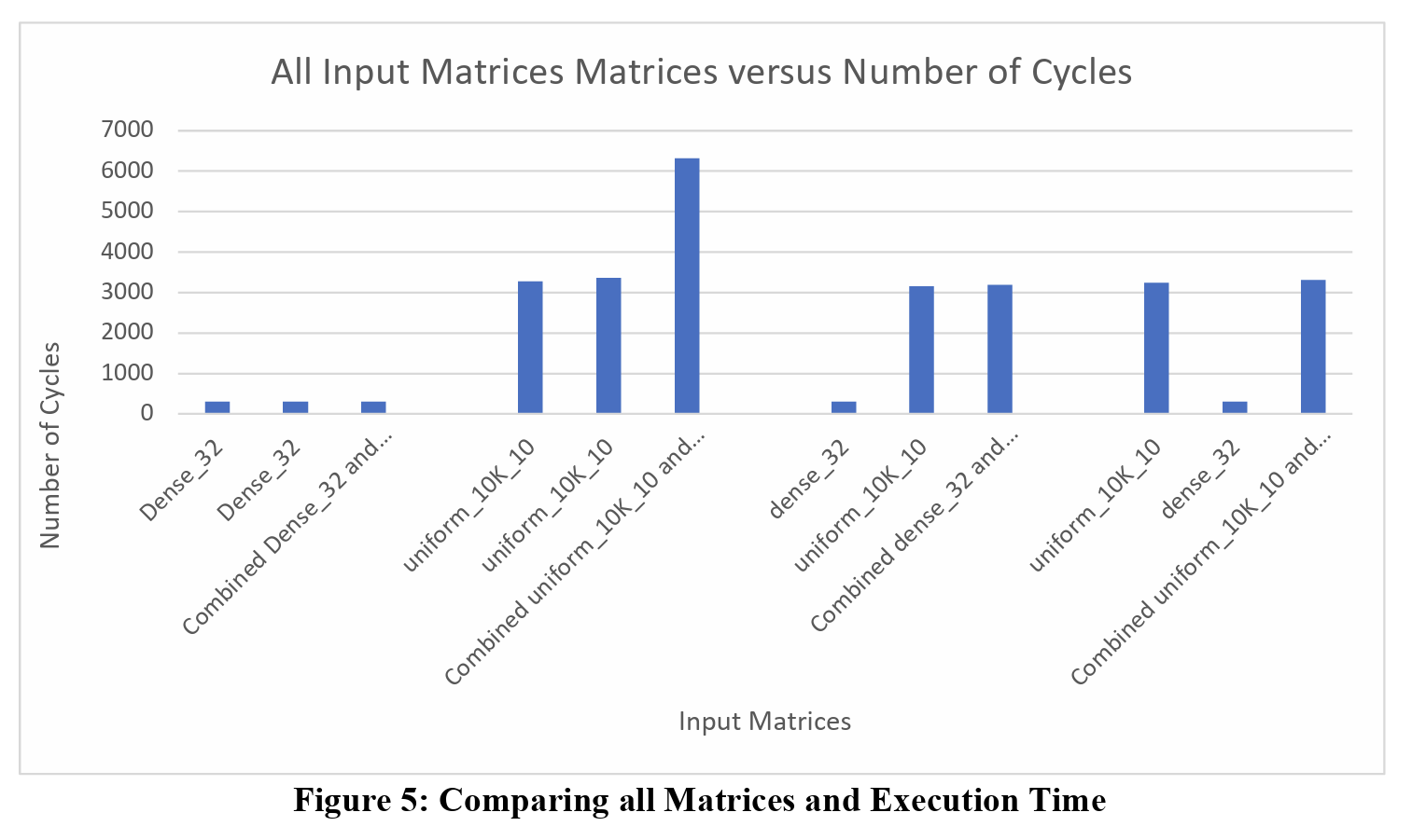
From this graph, we can see how the overall execution time for all combined matrices, except for the combination of two Uniform_10K_10 matrices, is the same as the larger of the two input matrices. The following figures highlight each combination, like Table 1 shows.

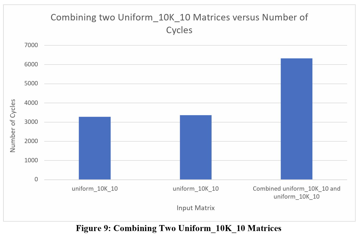
Just as the table highlights, all the combination matrices, except for the combination of two Uniform_10K_10 matrices, finishes execution at the same time as the larger input matrix, and there is a very good reason for this. Before loading the matrices and sending the inputs to the FPGA, the input matrices are row padded by a value of 8 times the number of HBM channels being used. This is done because in each SpMV cluster, there are 8 PEs that compute the result, and the number of HBM channels is dependent on the design.

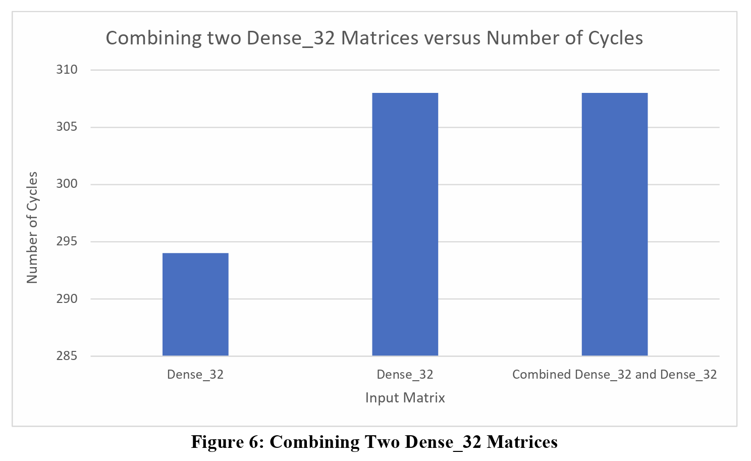
To properly test the comparison of the two inputs matrices and their combination, I need to appropriately pad each matrix. For the individual matrices, these inputs are padded to the closest multiple of 128, which is 8 times 16, the number of HBM channels used in this design. For the dense_32 matrices, when padded separately, these matrices will be padded to 128 by 128. When combined, their new combination will be 64 by 64, which will still be padded to 128 by 128. For this reason, the execution time will be very similar since the PEs are executing over the same number of elements as the individual matrices.

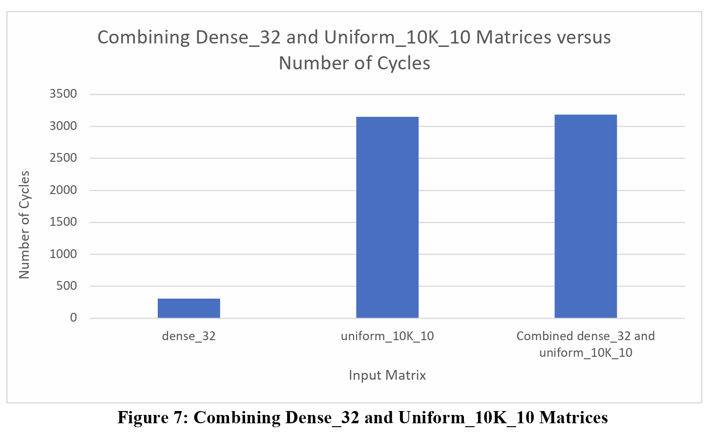
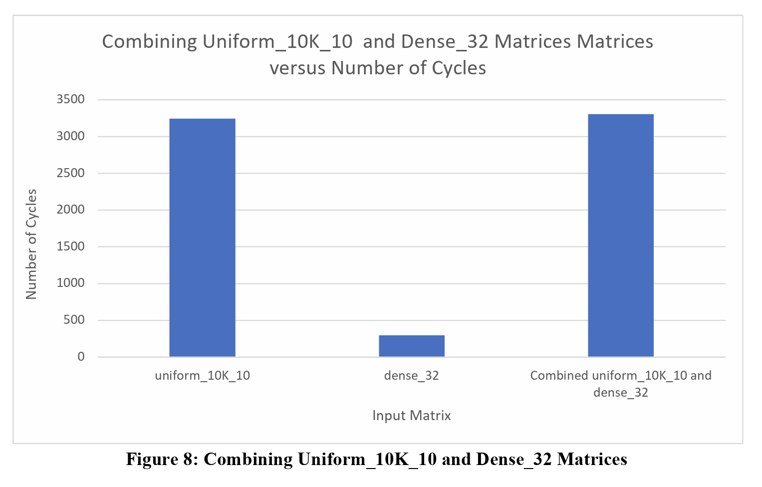
When combining dense_32 matrices and uniform_10K_10 matrices together, we still see very similar execution time with respect to the uniform_10K_10 matrix when compared to their combine matrix. The uniform_10K_10 matrix is padded to 10,112 by 10,112, as that is the closest multiple of 128 that’s greater than 10,000. Even when combining the uniform_10K_10 with the dense_32, we create a 10,032 by 10,032 matrix, within the same closest multiple of 128 as just the uniform_10k_10. If we were to combine another smaller matrix with the uniform_10K_10 matrix, say with a matrix of size 256 by 256, we could potentially see a more noticeable increase in execution time for their combined matrix.

However, unlike the other three combinations, when combining two uniform_10K_10 matrices together, we see a substantial increase in total execution time, almost 3,000 cycles more. This is to be expected though since we are now padding the combined matrix to a different size that’s greater than the two input matrices. As a result, more computation time is needed to compute all indices inside the matrix.

In order to decide if combining matrices is worth it, we should also considering the execution time in terms of microseconds for a given frequency. The table below highlights the overall time for different frequencies to get a better idea of how long users might be waiting in a large matrix is combined with a smaller one.

Input Matrices	50 MHz	70 MHz	100 MHz	200 MHz	300 MHz
Dense_32	5.9	4.2	2.9	1.5	1.0
Dense_32	6.2	4.4	3.1	1.5	1.0
Combined Dense_32 and Dense_32	6.2	4.4	3.1	1.5	1.0
uniform_10K_10	65.5	46.8	32.8	16.4	10.8
uniform_10K_10	67.2	48.0	33.6	16.8	11.1
Combined uniform_10K_10 and uniform_10K_10	126.3	90.2	63.2	31.6	20.8
dense_32	6.2	4.4	3.1	1.5	1.0
uniform_10K_10	63.0	45.0	31.5	15.8	10.4
Combined dense_32 and uniform_10K_10	63.7	45.5	31.9	15.9	10.5
uniform_10K_10	64.8	46.3	32.4	16.2	10.7
dense_32	5.9	4.2	2.9	1.5	1.0
Combined uniform_10K_10 and dense_32	66.1	47.2	33.1	16.5	10.9

Table 2: Execution Time in Microseconds for Different Frequencies

As Table 2 highlights, the total execution time follows the same patterns as the cycle count, but since these times are in microseconds, it makes sense to combine the matrices together. There is an inherit latency that is caused when sending the matrices from the host to the device and when the device sends the results back to the host, which are not present in the calculations done for calculating the number of cycles. Since these matrices are relatively small compared to other test cases, specifically one that’s 108,000 by 108,000 in size, that would take significantly longer than the 10,000 by 10,000. Unfortunately, given the long hardware emulation time for calculating that matrices execution time, that matrix is not shown in my tests.

However, it’s fair to reason that matrices of those sizes will take a much longer time to execute, so combining smaller matrices with a matrix that’s much larger, like 108,000 by 108,000 does not make sense. In future implementations, I would add logic that would calculate the number of rows and columns in the matrices and figure out a threshold number that would prohibit matrices from being combined in one of the matrices exceed that threshold number. With the given test cases, however, the performance deficit from combining the dense_32 matrix with the uniform_10K_10 matrix is small and would combine these matrices together.

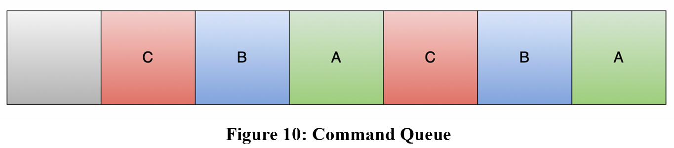
With the baseline design working successfully and given the positive testing information, future implementations can iterate on this design in the following ways, though not limited to just these. The first implementation would be to use OpenCL to split the matrix vector computation onto different sub-kernels so multiple matrices can be loaded at once. This requires a Command Queue that would handle any dependencies between user matrices and sub-kernels. Figure 10 below shows a basic command queue of the input matrices.

As the timing diagram from the baseline design shows, only one combined matrix can be executed at a time with the current design. However, figure 11 below shows a new timing diagram of what the system could look like with this new design.

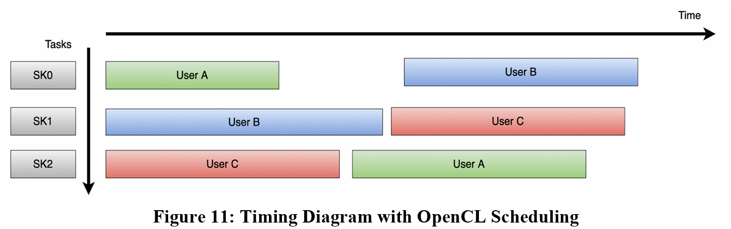
With multiple matrices now executing in parallel, we’d expect to see higher throughput, allowing users to get results faster, especially with higher demand. As shown in the timing diagram, the command queue would handle which user’s input goes to which sub-kernel. We can also notice some dependencies that OpenCL would handle, specifically with which each user’s matrix. In the diagram, I tried to show that there will still be a latency incurred by having to send data from the FPGA back to the host. This is why User A’s second matrix starts executing on sub-kernel 2, after user C’s matrix finishes. The same logic is applied to User B and C’s second matrices, where they are out of order when compared to the command queue, but that’s the benefit of using OpenCL for the scheduling as it will handle these operations.

Another consideration is the use of the baseline in the design using OpenCL for scheduling. As an example, if User A submits three matrices, two of which are 32 by 32, and one which is 10,000 by 10,000, we could combine the two 32 by 32 matrices together and avoid a third execution all together.

The main objective of my project was to implement as many HBM channels as possible into the GraphLily design as well as create a baseline system that can be used in a multi-tenancy system to allow multiple users and inputs to be computed in together to increase the overall throughput. Ultimately, I was successful in implement up to 26 channels and created a multi tenancy system where two matrices could be combined together which impressive results. While using 26 HBM channels, we were able to identify some key bugs that need to be solved, and were able to solve the SpMV bugs. While my evaluation testing was performed using only 16 HBM channels, we can assume that when including more channels, the overall execution time will decrease as there will be more processing elements working in parallel to help improve performance. While the hardware emulation runs a reference clock of 70 MHz, the actual hardware can run at 285 MHz. Once the hardware design is implemented on the FPGA and the device is running at this frequency, we can expect to see a significant decrease in execution time, just like Table 2 highlights. I look forward to seeing the next implementations of the multi tenancy system and what the team working on GraphLily can create.

1. Hu, Yuwei, et al. GraphLily: Accelerating Graph Linear Algebra on HBM-Equipped FPGAs.
2. N. Srivastava, et al. “Matraptor: A sparse-sparse matrix multiplication accelerator based on row-wise product,” Int’l Symp. on Microarchitecture (MICRO), 2020.
3. Y. Hu, et al. “GraphLily: Accelerating Graph Linear Algebra on HBM-equipped FPGAs” ICCAD 2021.
4. Y. Du, et al. “High-Performance Sparse Linear Algebra on HBM-equipped FPGAs Using HLS: A Case Study on SpMV” FPGA 2022.
5. X. Chen, et al. ThunderGP: Resource-Efficient Graph Processing Framework on FPGAs with HLS, ACM TRETS 2022.