ECE 3400: Intelligent Physical Systems

Electrical and Computer Engineering - Embedded Systems and Computer Architecture

In order to initialize the photoresistors, we needed to first focus our attention to how the arduino inputs and outputs data based on the pin layout. For our arduino to accept the inputs, we used pins A0 and A1 to read the values returned by the photoresistors.

In order for the Arduino to correctly read the values coming from the photoresistors, we coded a file we called, CdS_ReadA0A1. This file is used to analyze the difference between the two photoresistors connected to our robot to determine which side the light is in relation to the robot. These values, known as Normalized Measurement, were used in a ratio to tell the arduino which size has more exposure to the light. As a result, the arduino is capable of determining which side to turn to when the motors are connected in the next lab.

In the following two pictures and video, I will address our design choices and how the code works with respect to changing light intensity. In the video below, we see how as I move my flashlight from one side of the robot to the other, the intensity on the photoresistors change, changing values outputed by the sensor values and the Normalized Measurements.

CdS_ReadA0A1 Output:

Side view of the Robot:

From this angle, all components are clearly visible and the final shape of the light sensing robot is coming together. The large black wheels on either side of the robot will be commanded by the Arduino, while being powered by the 3 AA batteries and 9V battery underneath the breadboard. In the next lab, we will be connecting all of these together into the breadboard to get the Arduino powered, even when not connected to a computer via USB. The 3 sets of black and red wires shown in this image pertain to the 3 AA batteries connector, 9 volt battery, and the connector for one of the wheels. The other connector is out of frame. All of these will be connected to the breadboard in the next lab.

Top Down view of the Robot:

This top down image of the robot shows how the photoresistors were wired to correctly connect with the Arduino. The Arduino powers the board from the red, straight wire bridge instead next to the pin with the white markings around it. This pin outputs the necessary 5V the system needs. Given the versatility of the breadboard, I was able to connect everything correctly, only using the long colored wires when I needed to connect one side of the breadboard to the other. Otherwise, I used straight bridge wires to keep the board clean and contained.

The first step in getting our light following robot working is to set up the H-Bridge installed on our breadboard. The H-Bridge is used to control the wheels, with respect to the orientation of the spin as well as the speed of rotation. In the image of the H-Bridge below, I can see what connections I needed to make as well as where they needed to be connected to.

First, to power the H-Bridge, I needed to connect to chip to power, which is done through VCC1 and VCC2. These pins are connected to 3 AA batteries underneath the breadboard, giving them their own separate power source from the arduino. Both pins are directly wired to the positive rails of the breadboard. Next, to allow for direct control over the wheel speed, I needed to wire the enable pins: ENA and ENB to the PWM pins of our arduino. IN1 and IN2 were connected to the arduino, which I set to be either HIGH or LOW depending on whether I wanted the wheels to spin forward and backward. I followed the same steps for IN3 and IN4. To move the wheels forward, IN1 and IN3 were set to HIGH, while IN2 and IN4 were set to low. To go backward, the HIGH and LOW values are switched. In order to send the values to each wheel, OUT1 and OUT2 corresponded to the IN1 and IN2 values respectively. The same is done for OUT3 and OUT4. Setting these values in the output pins allows the wheels to move in the direction I desire. Lastly, the 4 ground pins are directly connected to the ground rails of the breadboard.

Now that the H-Bridge has been correctly set up, the next step is to calibrate the motors of the wheels. As with all manufacturing, every part is slightly different, and in the case of the motors, setting the value of one motor does not mean both motors will operate at exactly the same speeds. To equalize the speeds of both motors so that the robot would move forward and backward in a straight line, significant trial and error was required to determine the appropriate values.

As one can see, when the robot moves forward and backward, the robots veers to the right, toward the edge of the table. At this point, both wheel motors were given the same motor speeds, which meant that I needed to figure out the correct values for each motor so the robot would move in a straight line.

In the video below, the robot now moves across my desk in a straight line. For this step, I set the wheel speed to be slow to check if the robot would veer to the left or right. Clearly, the wheels have successfully been calibrated and the robot slowly moves in a straight line across my desk.

Following the same calibration process as before, when I set the wheel speed to be faster, the robot moved faster than in the previous step, while still moving in a straight line. While this may not look straight, upon closer inspection, I realized that I had not positioned the robot perfectly horizontal to the edge of my desk and the center caster wheel was also off the center line, resulting in the robot moving closer to the edge of the desk, but still in a straight line.

Now that the wheels are working the way I need them to, the next step is to incorporate the photosensors so the robot will turn and move forward depending on the location of a light source. Using the same wiring diagram and pin layout from Lab 1, I reconnected the photosensors, shown in the images below. All wires are now connected, except for the red and purple wire shown to the side of the robot. This wire is connected to the 9V battery underneath the breadboard and is used to power the arduino when not connected to power through the USB cable.

As shown in the pictures above, I did some cable management of all the wires needed for the robot by using white twist ties. This not only bunched the cables together neatly, but also served to keep the wires away from the photosensors and prevent light from reaching them. If a wire was blocking light to the photosensor, the robot would not perform correctly.

The final step in making the robot work was coding the arduino to take the information from the photosensors and use it to determine how to move the robot. There were a few key tasks the robot needed to accomplish to make sure it worked as intended. When there was not enough light or too much light to determine which direction to turn, the robot needed to spin in place, flashing an orage LED indicating it is unsure where to go. Once enough light was provided, the robot would turn in the direction of the light and turn off the orange LED. Turning off the LED with this step is important when the robot turned in the same direction as it did during the spinning process when there was not enough light. Without turning off the LED, it would be hard to determine if the turning operation when following a light source was properly working. With this implementation, it became evident the robot was turning toward the light source and recognized that this was the direction it needed to turn. When turning in the opposite direction, it's very clear that the robot is turning properly as the spin of the robot switches directions. Lastly, the robot needed to move forward in a straight line. As one can see in the video below, the robot does exactly as I intended for it to do, and I successfully created a light sensing robot!

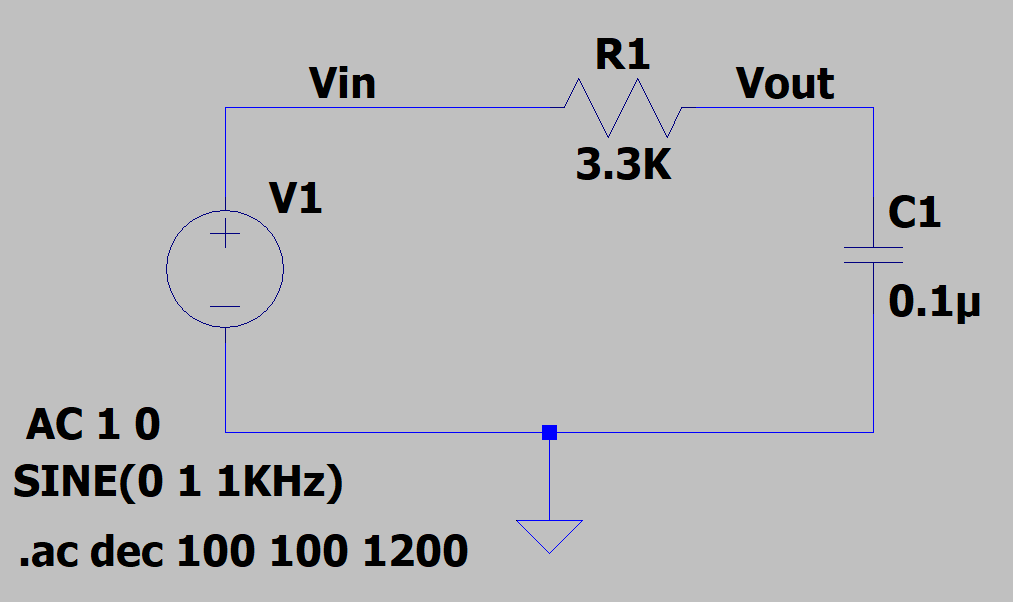
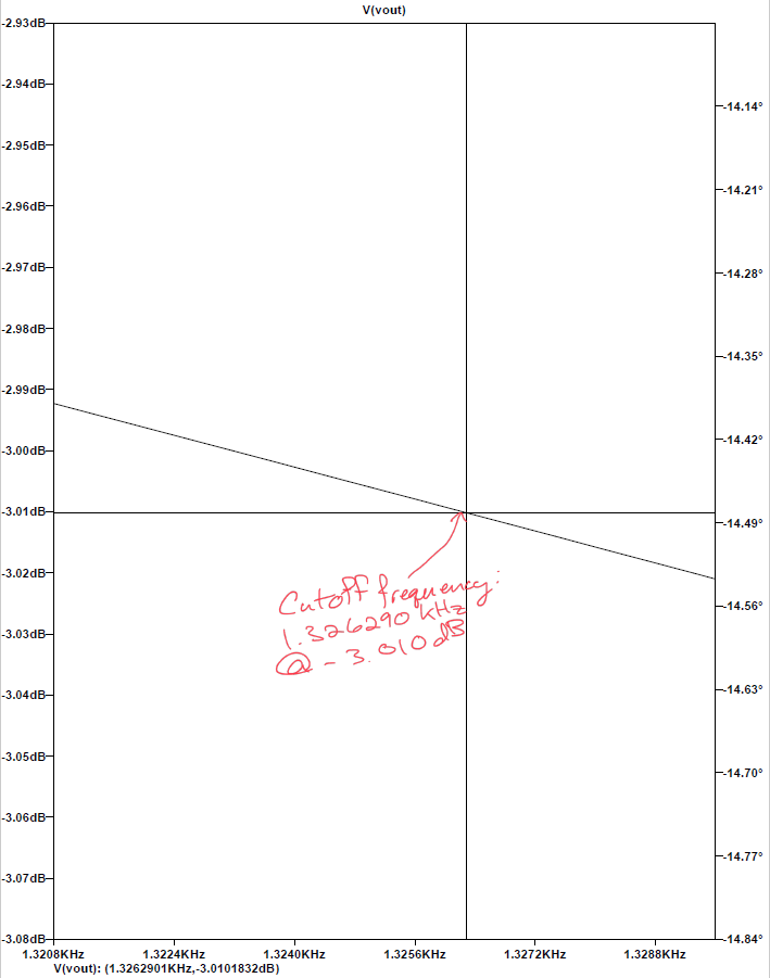
Using LTspice to simulate the cutoff frequency of the circuit, I was able to determine that the cutoff frequency of the circuit is at 1.3269 kHz. To calculate this, we use the formula 1/(2πRC). In this case, the resistance, R, is 3.3k Ohms, and the capacitance is 0.1 microFarads. In the image below, we can see the cutoff frequency right at -3.0 dB.

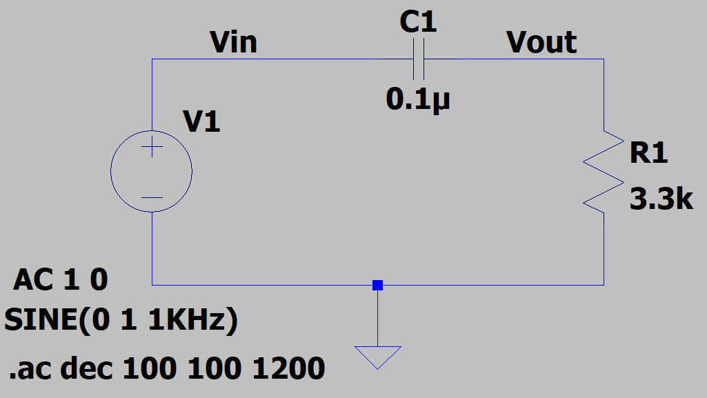
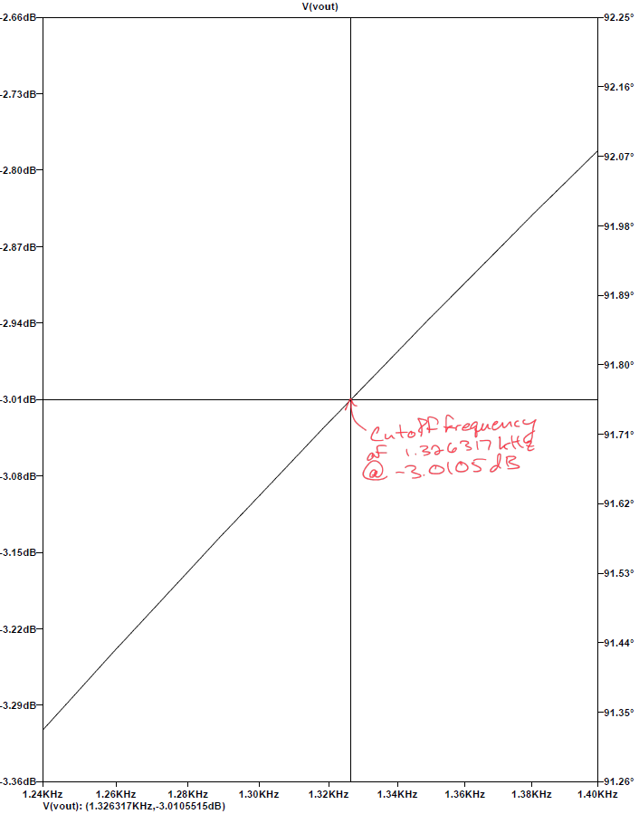
Just like with the Low Pass Filter and using LTspice to simulate the cutoff frequency of the circuit, I was able to determine that the cutoff frequency of the ciruit is at 1.3269 kHz. Using the same formula for the Low Pass Filter, the cutoff frequency is the same and we can see that the frequency cuts off at -3.0 dB.

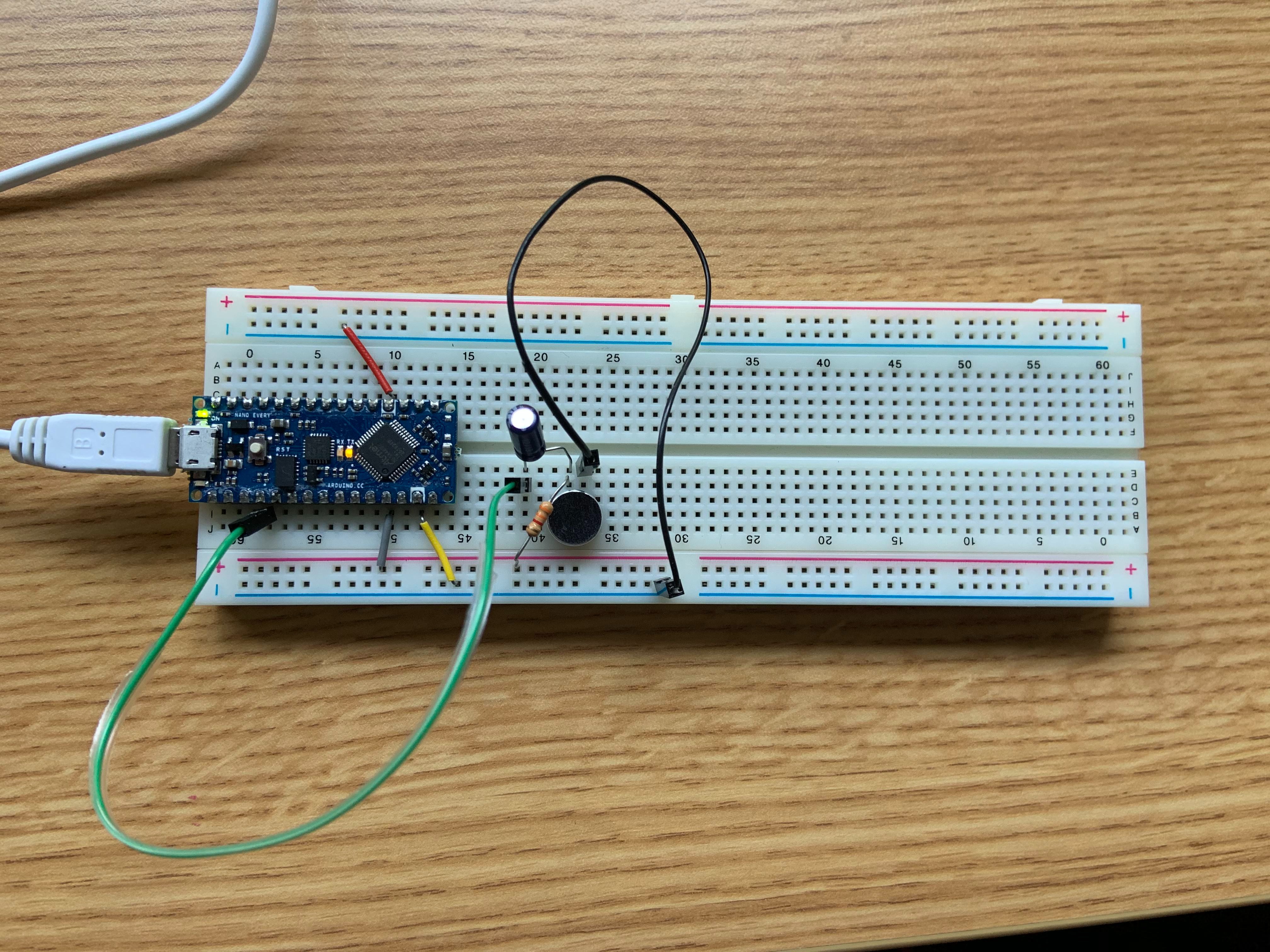
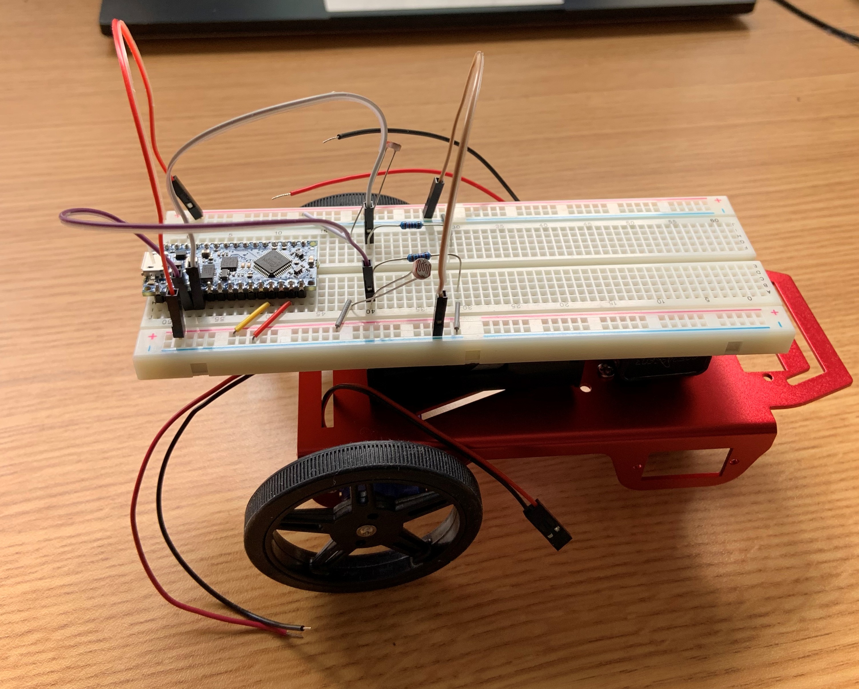
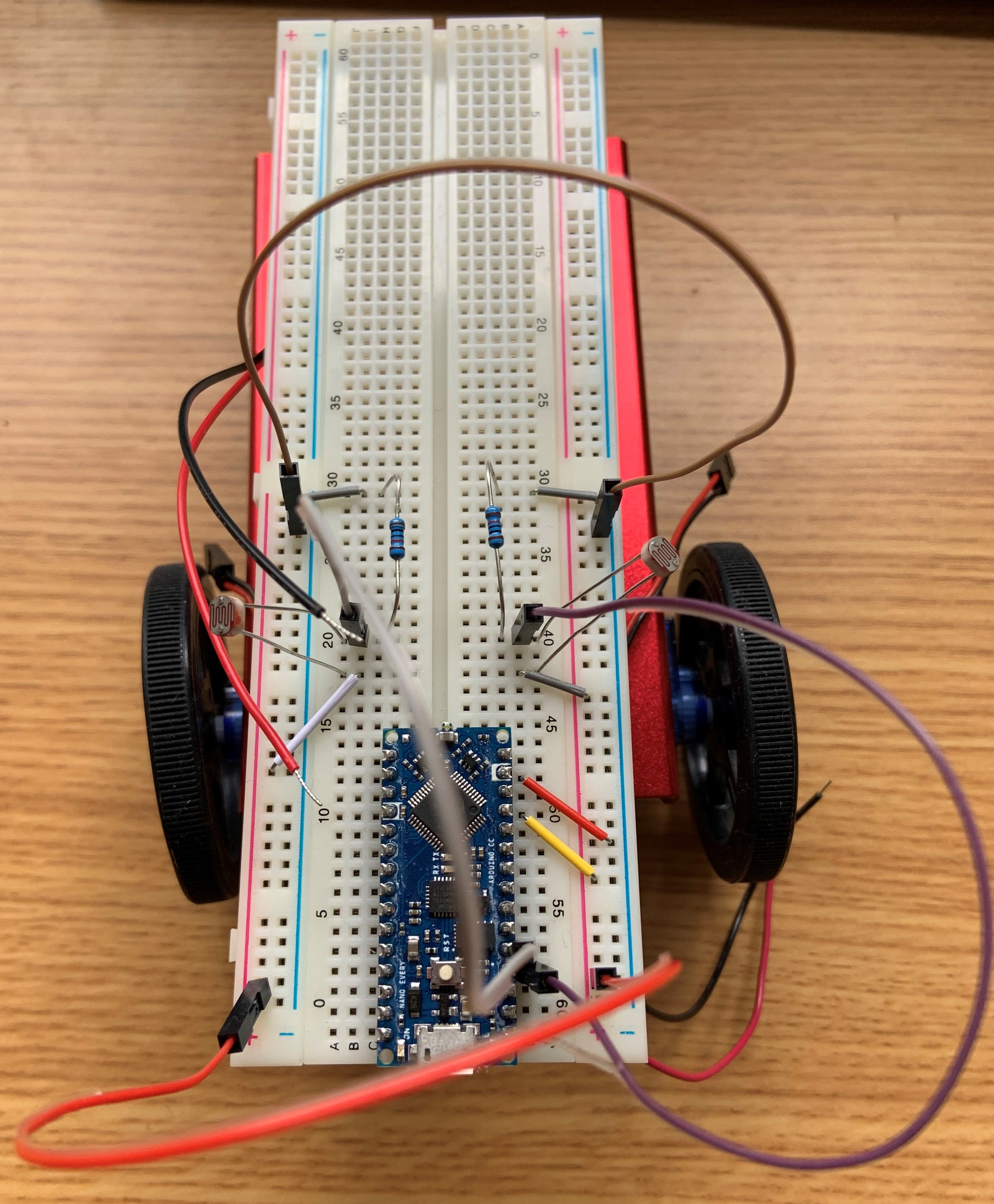
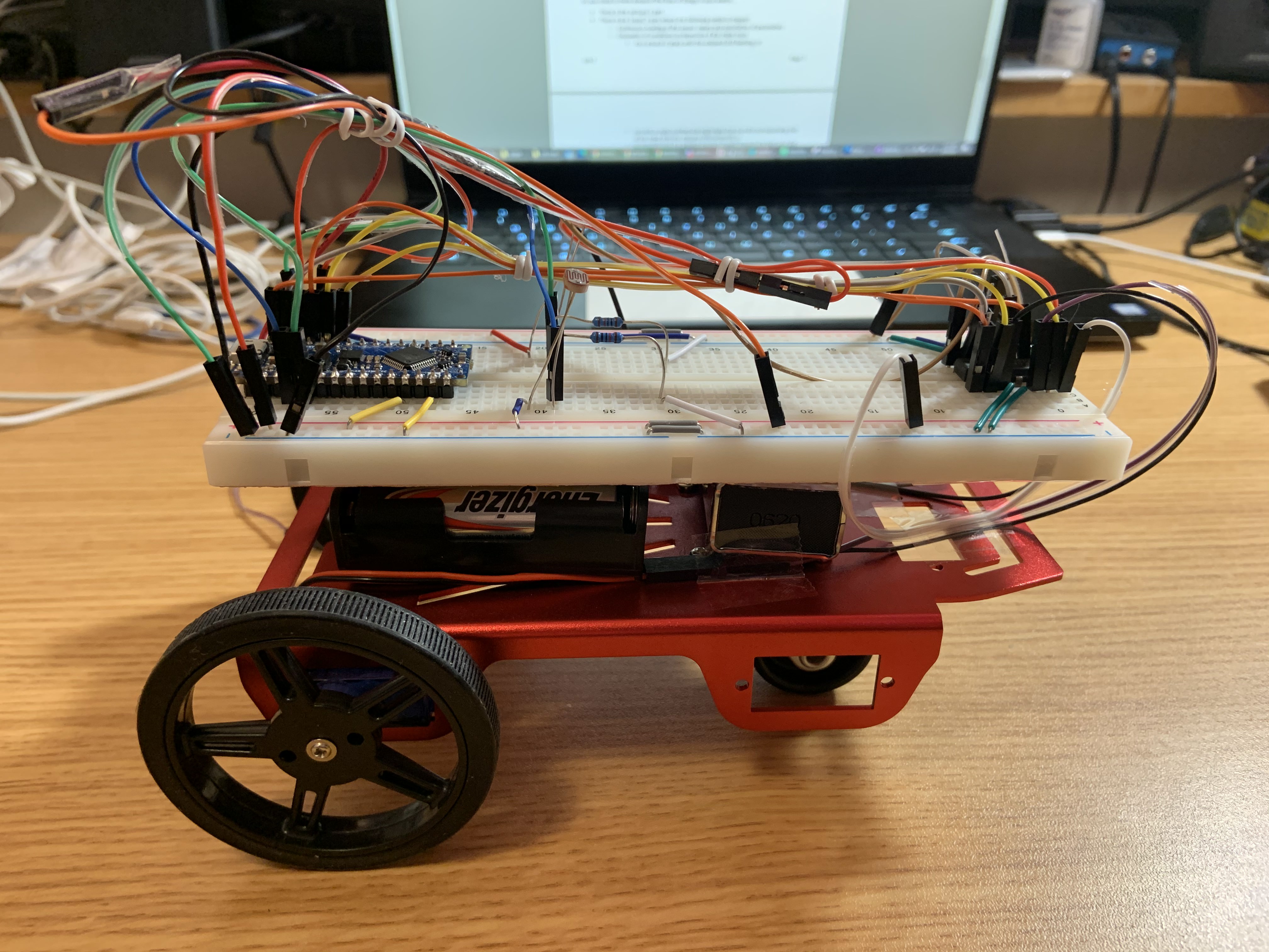
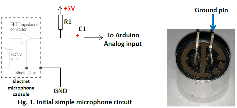
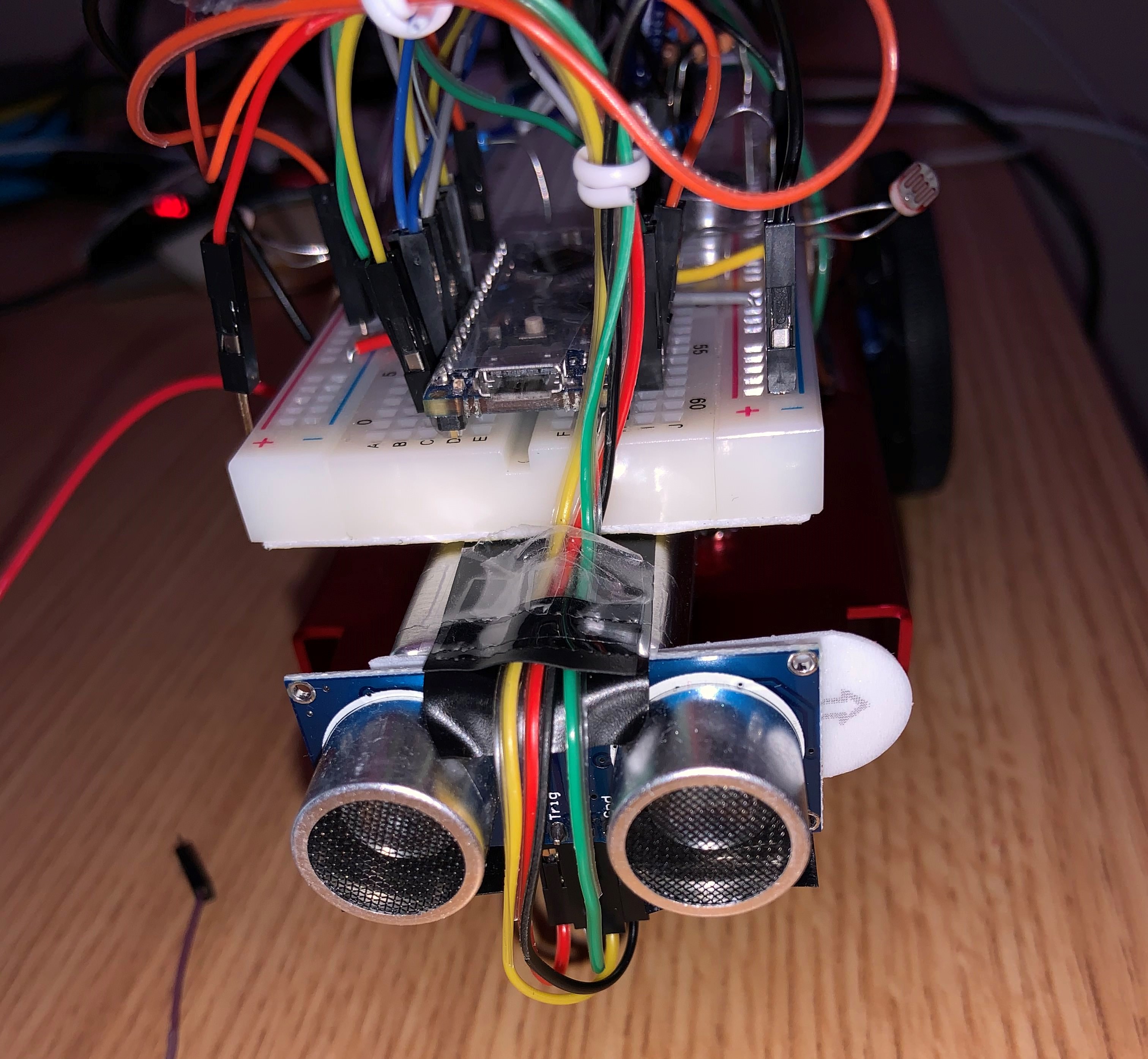
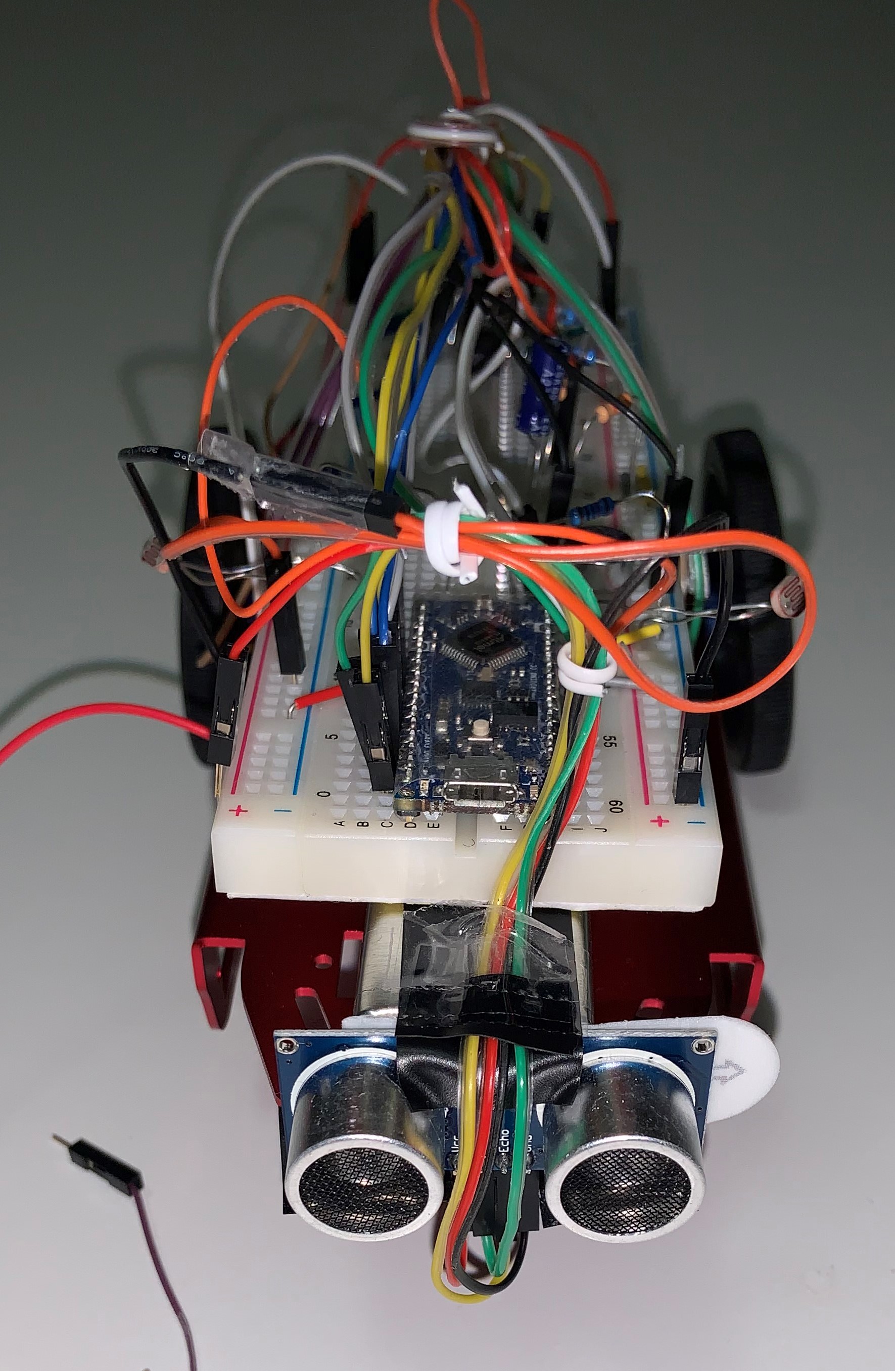
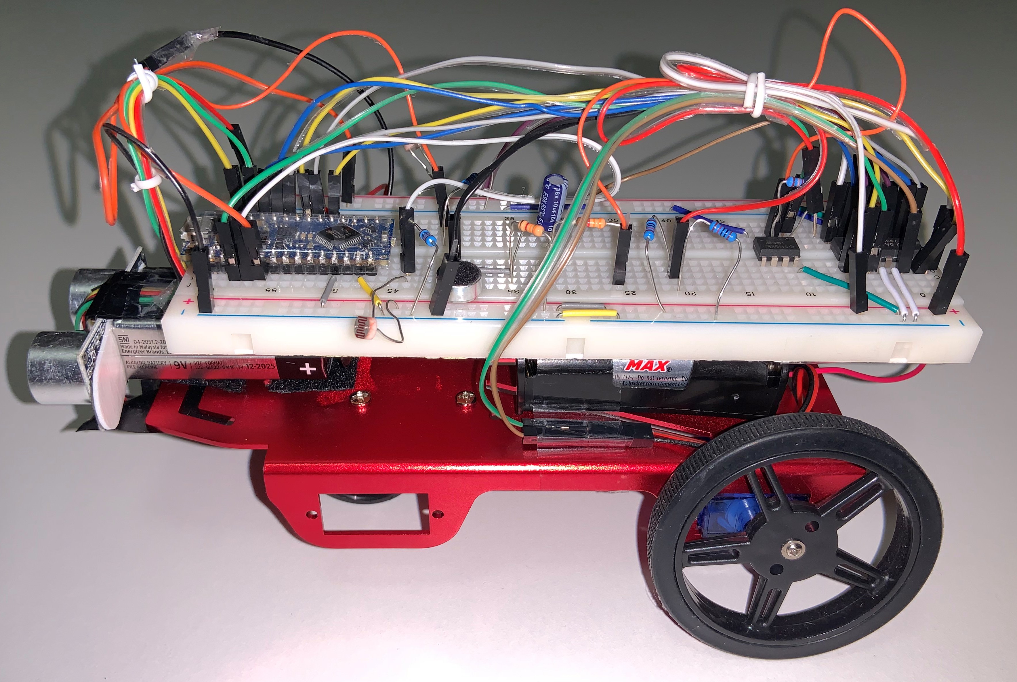
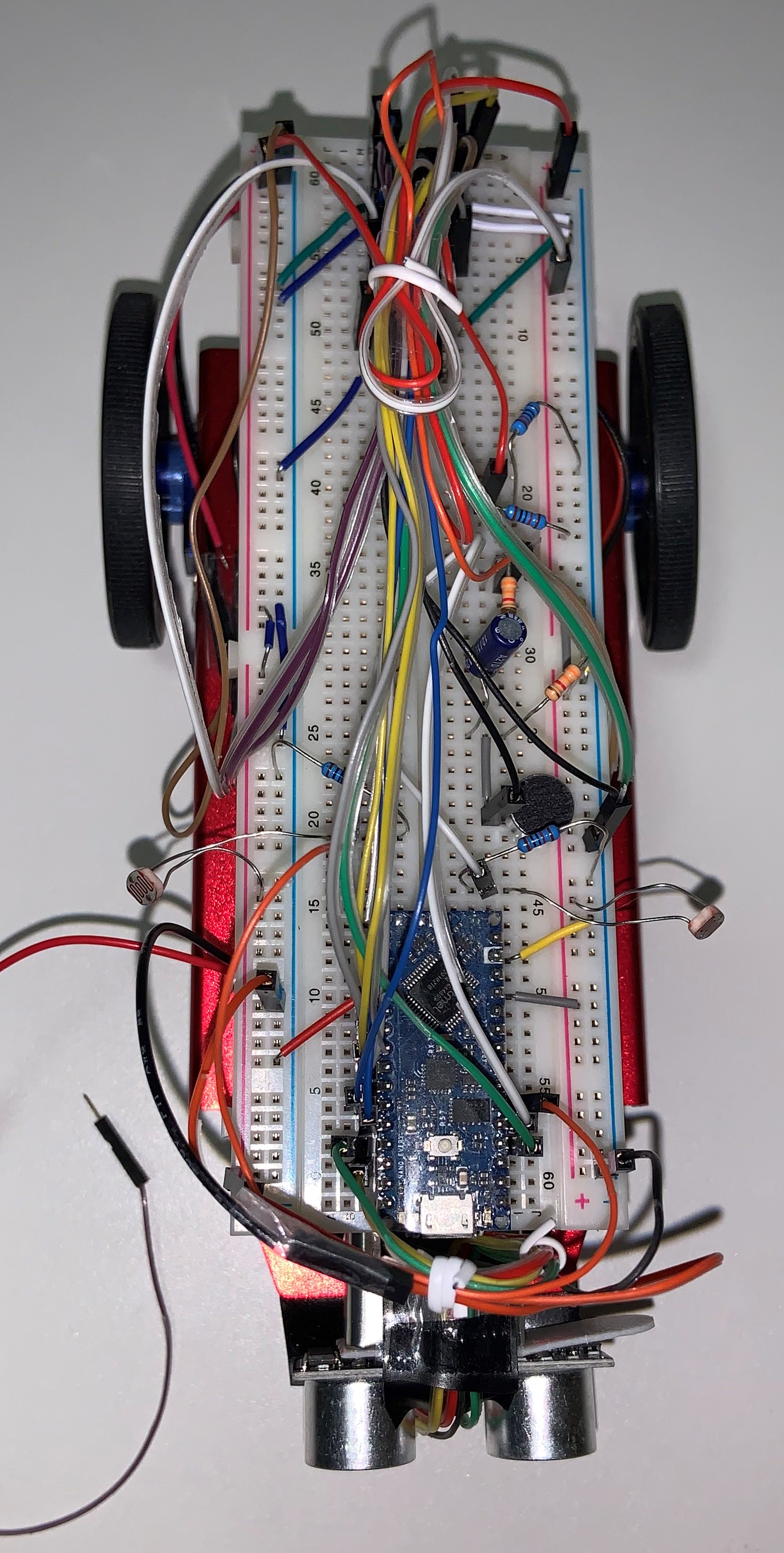
To connect the microphone to the circuit, I needed to accomplish several tasks. The first and most important thing is to connect all Arduino grounds, shown in the red and yellow wire bridges. I also had to connect the Arduino to the positive rail by using the gray wire bridge. From here, it was time to set up the microphone circuit. In the schematic below, it is important to assembly carefully and correctly. In my circuit, I positioned the microphone in the same orientation as shown in the image below, with the ground pin on the righthand side. On the left side of the microphone, I connected a 3.3k Ohm resistor as well as a 10 microFarad capacitor. The resistor is connected to the 5V rail, while the capacitor is directly connected to the A0 pin of the Arduino using the long green wire cable.

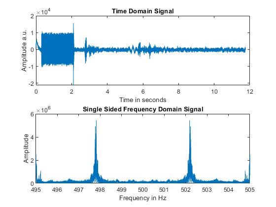
While I cannot release my code, it is important to discuss the following the steps I followed in order to get my code to work: complete the setup function, initialize ADC0 to the correct pin output value, create a boolean function to tell my loop function if the conversion is done, create a reading function to read the vale of ADC0, and the loop function which took the input values from the microphone and converted them to signed 16 bit integers for easier analysis. In addition to coding the Arduino, I also used a MATLAB program to play a sound at 500 Hz and collect the data directly from the Arduino. With this data, I was able to plot the Time and Frequency Domains collected by the Arduino. The image below shows the result of this data.

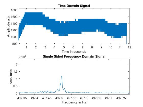
As one can see in the Frequency Domain graph, the peak frequency is not at 500 Hz, but rather after 497.5 Hz. This can be a result of many factors, especially differences in the manufacturing process that can skew data just a little bit. As a result, even though my peak frequency is seen at just after 479.5 Hz, this is still an acceptable result as it is very close to 500 Hz.

As one can see in the Frequency Domain graph, the amplitude of the peak frequency is rather weak, making it hard to differentiate from the other frequencies. To remedy this, I needed to build an amplification circuit to boost the amplitude.

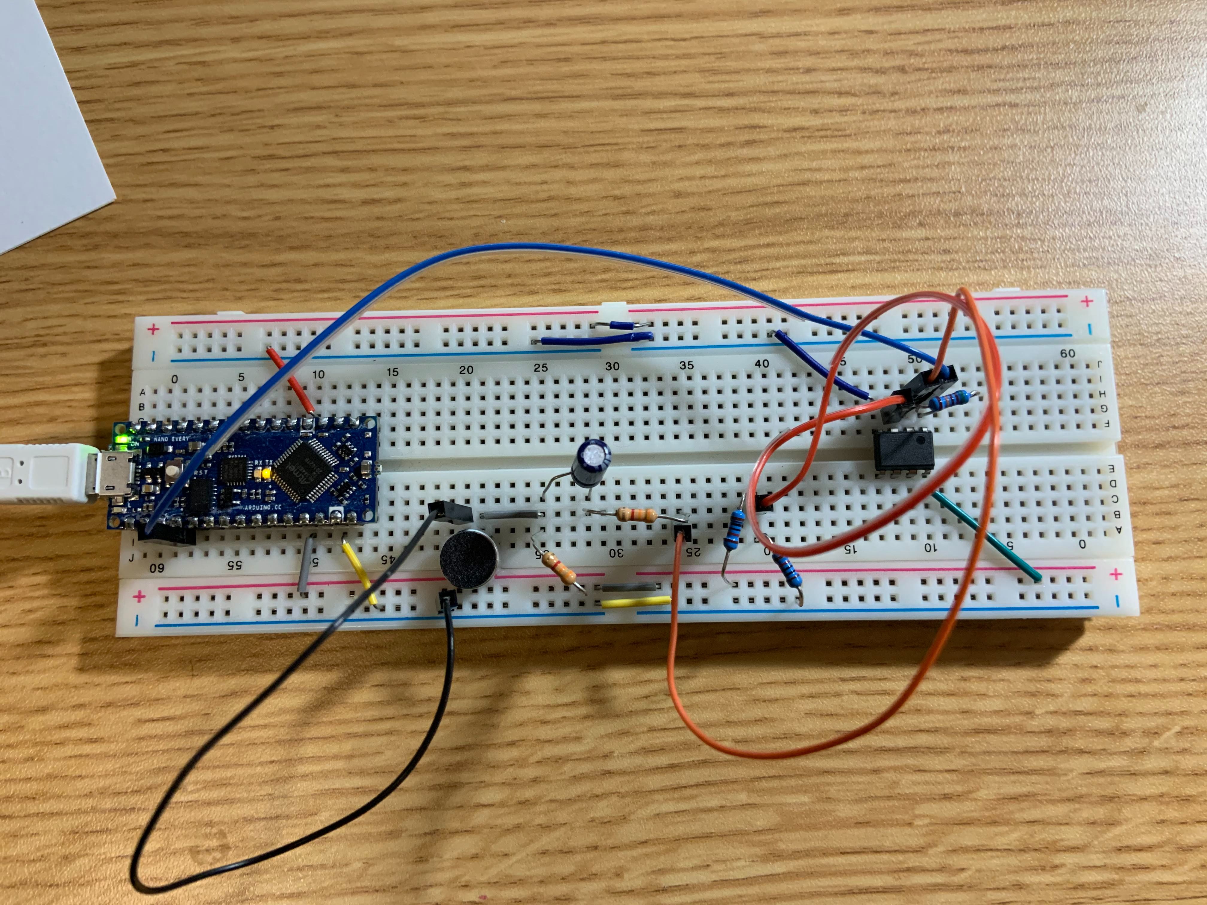
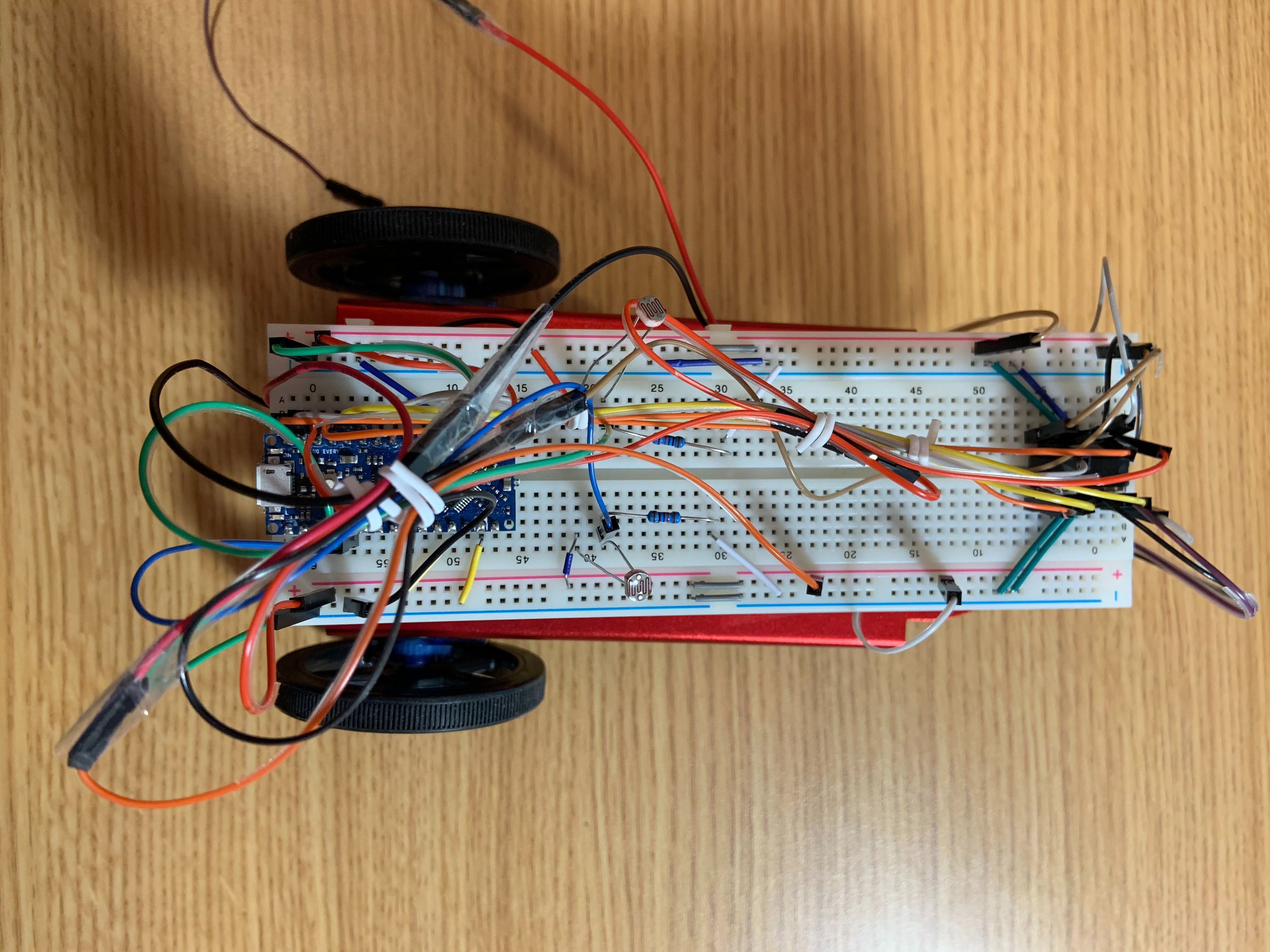
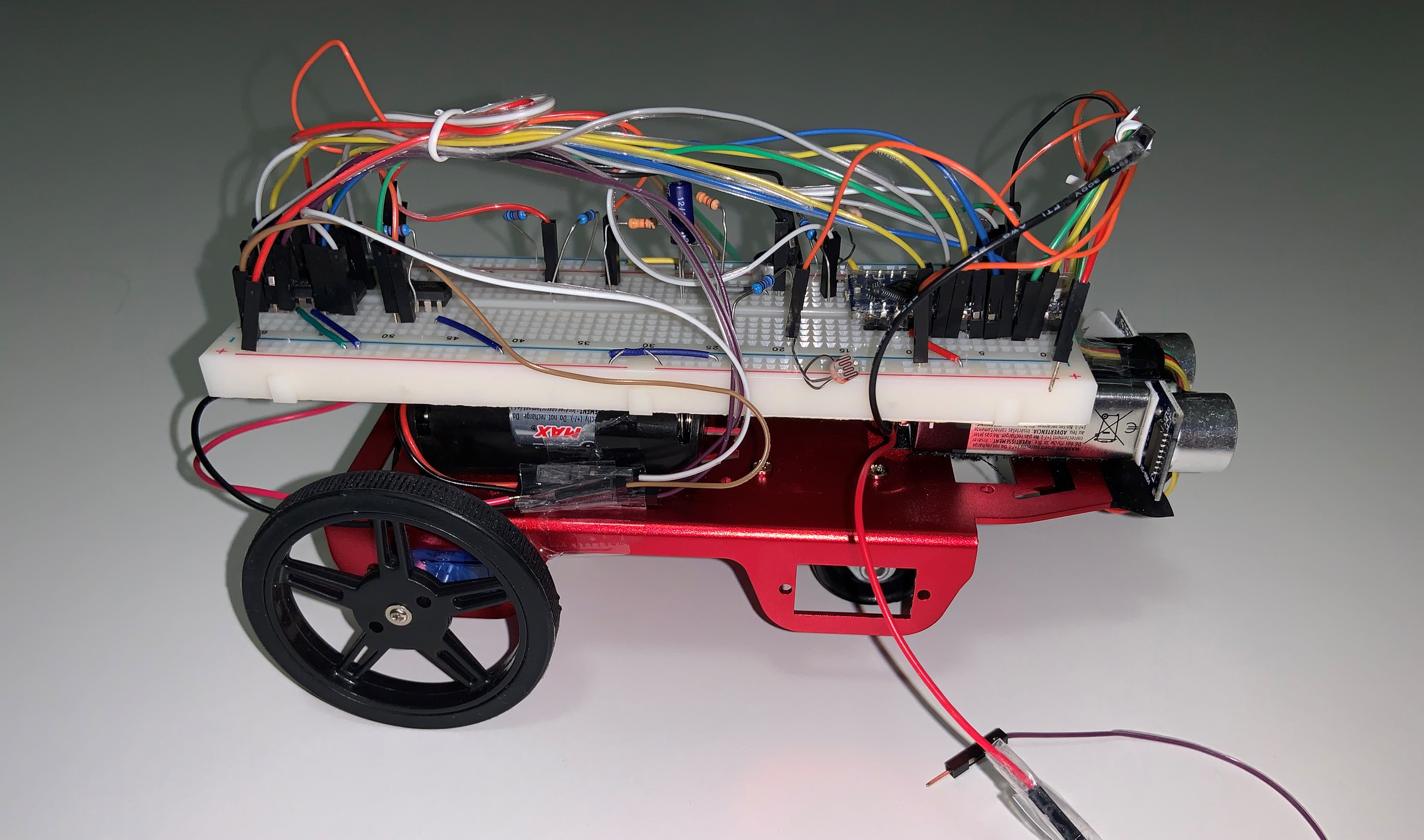
In the image above, one can see the amplifaction ciruit to the right of the microphone. Unlike in the first circuit, I decided to flip the position of the microphone, so now the negative, or ground, terminal is on the left, while the positive terminal is on the right. This was a necessary change to minimize the use of cables and make wiring this part of the circuit easier and more intuitive. In order to make the amplifier circuit work, I needed to make a few changes. Using the schematic shown below, one can see what was needed to be done.

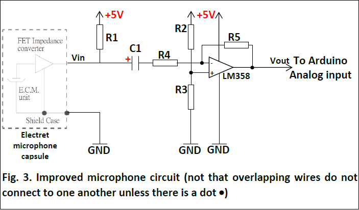
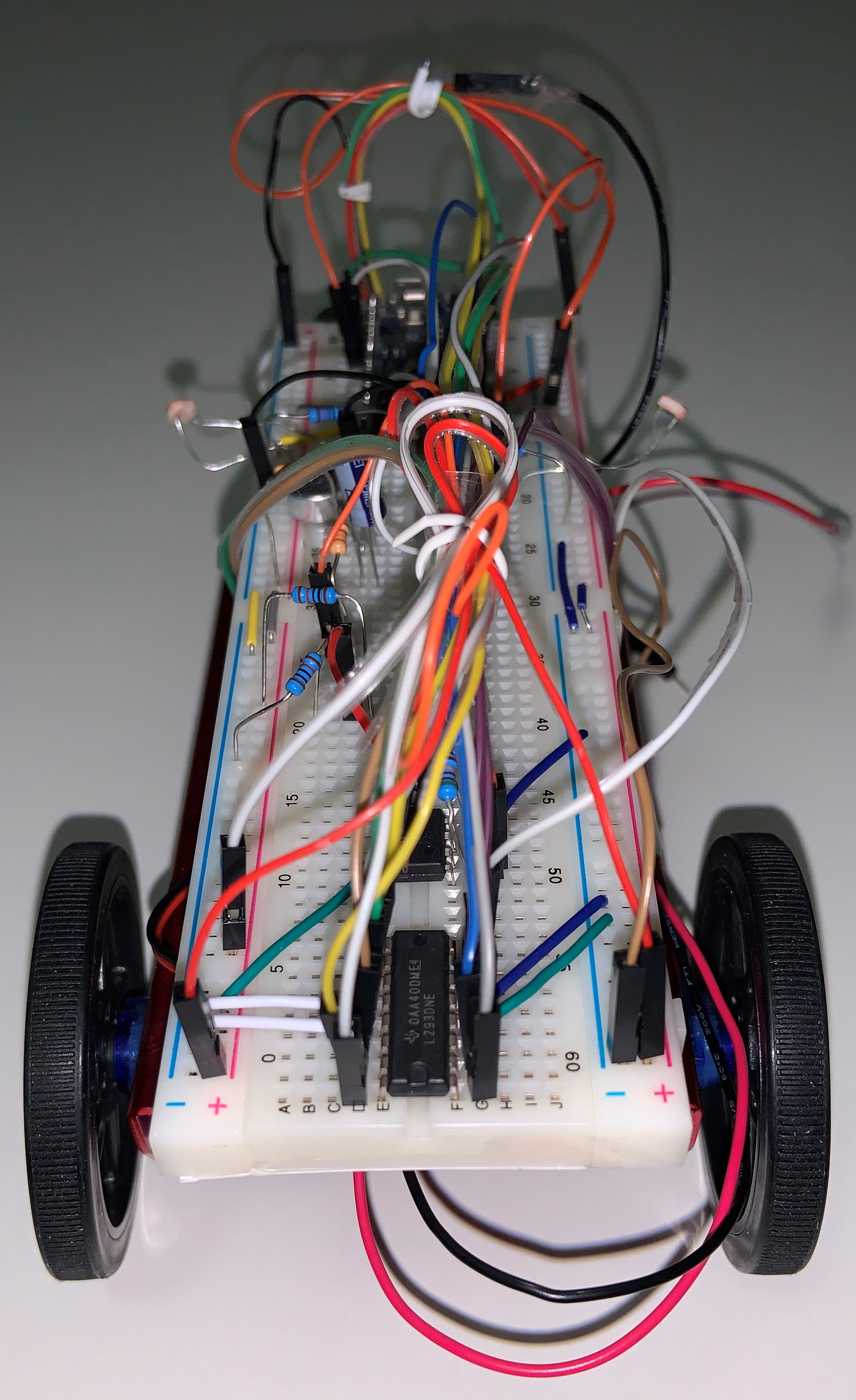
Using a LM358 OPAmp, two 3.3k resistors (R1 and R4), two 10K Ohm resistors (R2 and R3), and one 511K Ohm resistor (R5), I was able to successfully build the circuit, as shown above. In the OPAmp, I needed to connect both ground terminals, as well as the correct V- and V+ terminals. The negative terminal was connected directly from R4, while the positive terminal was connected from the terminal between R2 and R3. R5 was connected between the input into the negative terminal and the output leaving the OPAmp. As a result of this amplification, one can now see two, much larger, peaks in the frequency domain.

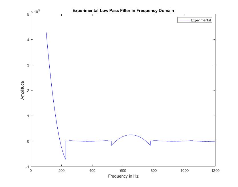
In order to test whether a Low Pass or High Pass Filter would be better, I simulated the two in LTspice. Using the simulated and experimental data, where the experimental data was collected from building the Low Pass circuit on the breadboard, I was able to determine how the input noise affected the output. When looking exclusively at my experimental data, the MATLAB program I used earlier produced the following graph.

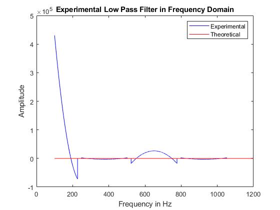
When combined with the simulated data, it becomes hard to conclude whether using the Low Pass Filter is a good choice as a lot of noise remains.

As a result of this data, the benefits of using a Low Pass Filter are unclear and I needed to test a High Pass Filter to see if I would get better results.

After not being able to tell if a Low Pass Filter had any beneficial impact on my circuit, I simulated the High Pass Filter in LTspice again. Following the same steps and using the simulated and experimental data, where the experimental data was collected from building the High Pass circuit on the breadboard, I was able to determine the theoretical output of the circuit. When looking exclusively at my experimental data, the MATLAB program I used produced the following graph.

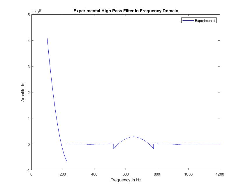
At first look the similarity of the graphs was confusing, but when I scrutinized them more closely side by side, I determined that the High Pass Filter providing less overall noise. This is a better filter, but still introduces noise into the circuit. This becomes more clear when we compare the experimental data with the theoretical data, just as I did with the Low Pass Filter.

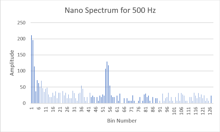
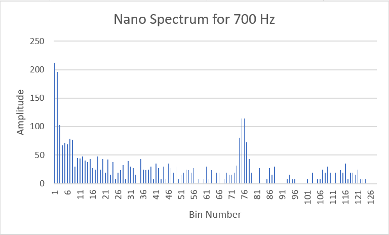
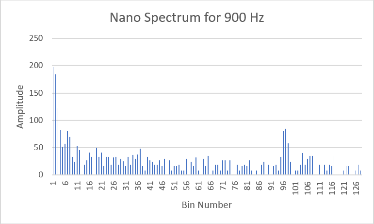
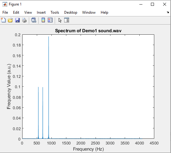
To get the FFT functions working on the Arduino natively, I needed to install the FFT library downloaded directly from this link. Once added into the Arduino's library, I coded the final part of the lab, by incorporating the FFT functions so when a sound was played, the Arduino would automatically output the FFT of the sound generated. In the following images, I will show the FFT of a 500 Hz sound, as well as a sound played at 700 Hz and 900 Hz.

Clearly, my FFT implementation works just like it should, with different peaks depending on the frequency. In the 500 Hz FFT, the peak amplitude is close to bin number 50, while in the 700 Hz FFT, the peak amplitude is close to bin number 70. Finally, in the 900 Hz FFT, the peak frequency is a little to the right around bin number 96.

To attach the ultrasonic sensor, I used 3M poster tape and electrical tape to secure it to the front of the robot. While instructed to use velcro strips to attach, I did not have any velcro left so using the 3M poster strips was a great alternative because the foam is a great insulator. Also, as I did not want to accidentally short the sensor, I needed a proper insulator to keep it safe. I also used the electrical tape to help secure the sensor and the wires needed to connect the sensor to the Arduino. In the images below, one can see how I attached the sensor to the robot.

Now that the ultrasonic sensor has been attached to the robot and connected to the correct pins on the Arduino, I needed to measure the readout from the sensor and determine the accuracy. To do this, I placed the robot a set distance away from an object, in this case a small box, to test the read out of the sensor in comparison to the actual distance. I tested at multiple distances, including 2, 4, 6, 8, 10, 15, 20, 30, 40, and 50 centimeters away from the robot. The graph and table below illustrate how accurate the sensor is.

Actual Distance	Recorded Distance	Error
2 cm	3.26 cm	1.26 cm
4 cm	4.51 cm	0.51 cm
6 cm	6.24 cm	0.24 cm
8 cm	8.39 cm	0.39 cm
10 cm	10.19 cm	0.19 cm
15 cm	15.99 cm	0.99 cm
20 cm	21.15 cm	1.15 cm
30 cm	29.96 cm	0.04 cm
40 cm	40.61 cm	0.61 cm
50 cm	50.64 cm	0.64 cm

For this demo, I will have the robot spin in a circle and flash the onboard LED whenever it detects an object. I will also have the robot use the included microphone and amplification circuit to start spinning when a 550 Hz signal is produced. Using my iPhone to play this sound, the robot began spinning after recognizing and registering the 550 Hz input. The following images depict the path and orientation of the robot with respect to the objects as well as the frequency spectrum of the input signal.

In the video below, one can see when the robot passes the two obstacles, an orange LED flashes and after passing the second obstacle, the robot stops spinning, indicating that the robot registers it has passed both of them.

For Demo 2, I needed to add in the light sensors I used in Lab 1 and 2 - "Light Following Robot". For this demo, the goal is to move the robot toward an obstacle using a light source and have the robot stop once it gets within a certain distance from the obstacle. The following image shows the path the robot needs to take in order to complete Demo 2.

As shown above, the robot must start off to the right, not moving when there is no light source for the robot to follow. Once a light source is provided, the robot must turn left toward the first obstacle. Once the robot reaches the first obstacle, the onboard LED must be turned on and the robot must to turn to the right, not the left. This is evident in the video below where I show that the robot will not turn to the left, after reaching this obstacle. Continuing down the path to the right and toward the other obstacles, once the robot reaches obstacle 2, the onboard LED must turn back on again to indicate it now detects another obstacle. Once reaching obstacle 2, I turned the robot again to the left to face obstacle 1 again. The robot indicates that it detects obstacle 1 by turning on the onboard LED and continues to turn left to obstacle 3. Now that the robot has reached obstacle 3 and has turned on the onboard LED, the demo is done, demonstrating that the robot will stop when it detects an obstacle within a specified distance away from the robot. In the two videos below, the first video will zoom in to show the onboard LED turned on when it detects each obstacle and the second video will show the path the robot takes without zooming in and showing the LED.